Generating Risk Maps

library(mappestRisk)

Generating risk maps for pest development

Overall approach and ecological meaning

mappestRisk aims to provide an easy-to-use modelling workflow for producing pest risk maps.

Development rates variation across temperatures has been largely used to produce risk maps of pest occurrence, usually maps of annual generations for arthropod crop pests based on linear models (see e.g., (Health (PLH) et al. 2017)). Despite more complex approaches have been recently used for pest risk assessment based on biological responses to temperature(Health (PLH) et al. 2023), nonlinear TPC modelling of development rates variation across temperatures, already available after decades of experimental data collection, can help inform pest risk assessment throughout multiple crop pests¹.

The approach followed by mappestRisk is inspired by the one developed by Taylor et al. (2019). These researchers compose a mathematical model through TPC model fitting that describes the temperature-dependence of huanglongbing transmission from Diaphorina citri to citrus plants. Given that this model theoretically approximates the fundamental thermal niche of the species, they project throughout citrus growing regions how many months per year have average temperatures that result optimal for transmitting the virus. This index (number of high risk months) results extremely helpful for policy making, since it reduces sources of uncertainty in the communication field by using a direct, applied measurement (Simmonds et al. 2022).

Given the major contribution of development rate TPCs to ectotherms’ fitness(Pawar et al. 2024; Amarasekare and Savage 2012) and thus likely on fundamental thermal niche, here we suggest applying a similar framework in a simpler way to calculate how many months per year are optimal for a population to maximize its development.

Calculate the Thermal Suitability Boundaries

In order to obtain thermal suitability boundaries or limits defining the TPC region where development is maximum, the package incorporates the therm_suit_bounds() function.

This function has as input the tibble obtained after using the predict_curves() function, either with- or without uncertainty propagation. Note that only one model can be used for calculating thermal suitability boundaries at a time. Additionally, it has a suitability_threshold argument to allow the user to specify which quantile of the TPC is being used. In other words, a suitability_threshold = .75 will calculate the two temperature values at which the TPC predicts a value $R(T_{75}) = 0.75\times\ r_\max$ , one at each side of the TPC peak. If multiple TPCs are given due to setting the predict_curves() argument propagate_uncertainty to TRUE, two boundaries will be calculated for each TPC. This function outputs a tibble with the thermal suitability boundaries for each curve.

Note that setting suitability_threshold to 0 will yield the thermal limits of the complete TPC, i.e., the $CT_\min$ and the $CT_\max$. While the map resulting from default (.75) or similar threshold measures indicates severe risk (populations may rapidly develop), maps from permissive measures such as critical thermal limits may rather indicate risk of the pest to find a refuge in the selected region.

Here we provide a example²:

#fit previously:
data("aphid")
fitted_tpcs_aphid <- fit_devmodels(temp = aphid$temperature,
                                   dev_rate = aphid$rate_value,
                                   model_name = c("briere2", "lactin2"))
#predict curves previously
preds_boots_aphid <- predict_curves(temp = aphid$temperature,          
                                    dev_rate = aphid$rate_value,
                                    fitted_parameters = fitted_tpcs_aphid,
                                    model_name_2boot = c("briere2", "lactin2"),
                                    propagate_uncertainty = TRUE,
                                    n_boots_samples = 10)

boundaries_aphid <- therm_suit_bounds(preds_tbl = preds_boots_aphid,       
                                      model_name = "lactin2",        
                                      suitability_threshold = 80) 

The output has the following aspect:

print(boundaries_aphid)
#> # A tibble: 11 × 6
#>    model_name suitability tval_left tval_right pred_suit iter    
#>    <chr>      <chr>           <dbl>      <dbl>     <dbl> <chr>   
#>  1 lactin2    80%              21         31.3     0.114 1       
#>  2 lactin2    80%              21.8       32.5     0.113 10      
#>  3 lactin2    80%              21.5       31.9     0.113 2       
#>  4 lactin2    80%              22.3       31.7     0.121 3       
#>  5 lactin2    80%              21.2       31.6     0.113 4       
#>  6 lactin2    80%              22.3       32.2     0.116 5       
#>  7 lactin2    80%              22.1       31.9     0.114 6       
#>  8 lactin2    80%              21.8       32.2     0.113 7       
#>  9 lactin2    80%              21.1       32.4     0.115 8       
#> 10 lactin2    80%              22.3       31.6     0.114 9       
#> 11 lactin2    80%              21.5       31.8     0.113 estimate

Project a risk map

Given the fitted TPCs and their calculated suitability thermal traits, mappestRisk enables to automatically generate rasters –terra::SpatRaster– at the targeting region to forecast summarizing the number of months per year with highly suitable temperatures for pest development.

This can be done with the function map_risk()

The workflow of the function is as follows:

1. Extract temperature data: When no temperature raster is provided by the user in the t_rast argument (default NULL), map_risk() automatically downloads temperature data from WorldClim historical data set using geodata (Hijmans et al. 2024) package, consisting in average temperature at monthly time resolution and a user-defined spatial resolution through res argument –our function uses 2.5 resolution or ~4.625km at the equator by default. If the region argument is a string with any country name available in data(country_names), the function calls geodata::worldclim_country(). Alternatively, if the region argument is either a SpatExtent, a vector with the numeric boundaries of this spatial extent or a sf or SpatVector object –i.e., polygons, the map_risk() function will download data for the entire world using geodata::worldclim_global()³.
2. Spatial operations: Once the temperature raster is available (either through user-input in t_rast or by downloading from WorldClim), the map_risk() function operates using terra R package for spatial operations such as cropping the data to the target region spatial extent and masking (if mask = TRUE). Next, map_risk() uses the input of the argument t_vals –which has to be a tibble exported from therm_suit_bounds()– to assign a value of 1 at those cells with monthly temperatures within the interval given by therm_suit_bounds() or 0 if not, yielding a raster with 12 layers (1 for each month) with 0’s and 1’s. Then, it automatically sums those values for each cell across the 12 layers to give a final SpatRaster with one layer whose values vary between 0 or 12, indicating the number of months per year with highly suitable temperatures –within the thermal boundaries from therm_suit_bounds() from TPC model fitting– at that cell, or in other words, the risk value. When more than one row is given in t_vals (due to multiple thermal boundaries after propagating uncertainty with predict_curves()), one “partial” SpatRaster is calculated by map_risk() for each pair of thermal boundaries. In this case, a final SpatRaster is generated with two values layers: the Risk layer that averages the risk value across partial rasters and the uncertainty raster that calculates the standard deviation across these partial rasters as an uncertainty risk measurement.
3. Visualization: despite the function yields a SpatRaster, it automatically plots the map representing the raster values whenever the plot argument is set to TRUE. This map is generated using terra::plot() and will have one panel showing the risk value –i.e., the risk raster layer– and, when parameter uncertainty has been included in the complete mappestRisk workflow, it will add a second panel showing the standard deviation of the risk value in acton palette –i.e., the uncertainty raster layer. Cells are coloured based on their values using bilbao and acton palettes from khroma package (Frerebeau 2025).
4. Interactive maps: map_risk() has an additional logical argument called interactive, default to FALSE. If set to TRUE, the output of map_risk won’t be a SpatRaster any longer but a leaflet object instead, and an interactive map with the above-mentioned layers will be generated using terra::plet().

The following sections show how to obtain risk rasters with default visualization given directly by map_risk(). Custom alternatives for map visualization are detailed in Customize your Risk Maps article.

Risk map: country

If we follow the workflow of the package in the examples elsewhere in this website, we can then create a risk map for a country. In this example, we will obtain it for Bhutan.

Since Bhutan is the official name included in mappestRisk::country_names and no t_rast is given by the user, the function will automatically download data cropped for this country. In this case, we will use

# Create a Risk Map for Bhutan

risk_rast_bhutan <- map_risk(t_vals = boundaries_aphid, 
                             path = tempdir(), # directory to download data 
                             region = "Bhutan",    
                             mask = TRUE,
                             plot = TRUE,
                             interactive = FALSE,
                             verbose = TRUE)

#> 
#> Computing summary layers...
#> 
#> Plotting map...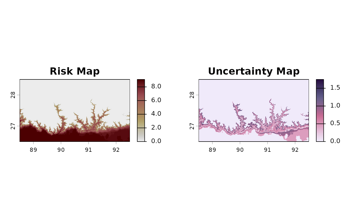

#> 
#> Finished!

The map on the left side shows how many months have optimal temperatures for the aphid Brachycaudus schwartzi along Taiwan, from 0 (in mountains and highlands) up to 9 (in southern lowlands). The map on the right side shows an error map from parameter uncertainties, with regions at which the risk estimate is exact (e.g., the mountains) and others with up to 1.6 yielding the standard deviation of the risk value (in number of suitable months) at specific cells.

Risk map: Spatial Extent

In the following example, the region will be a frame with four coordinates (xmin, xmax, ymin, ymax) encompassing the Bhutan projection that is used by default in map_risk() function. First, let’s convert the numeric extent into a SpatExtent using terra::ext()⁴:

bhutan_spatextent <- terra::ext(risk_rast_bhutan)

Then, we would apply the same function as before for the aphid workflow, with the new region argument set to "bhutan_spatextent".

risk_rast_bhutan_v2 <- map_risk(t_vals = boundaries_aphid, 
                                path = tempdir(), # directory to download data 
                                region = bhutan_spatextent,    
                                mask = TRUE,
                                plot = TRUE,
                                interactive = FALSE,
                                verbose = TRUE)

Risk map: Polygons

A typical scenario may involve forecasting data to regional or province level, to natural protected areas or to crop’s growing regions. In these cases, the user input for region must be an sf object –e.g., by loading a shapefile (*.shp) in R using sf::st_read()– or as a SpatVector –e.g., by loading a shapefile using terra::vect(). The map_risk() function will automatically download global data and crop it to the spatial extent of the object, and will perform a masking operation if mask = TRUE.

In the following example, we will use it for Bhutan, as well. The map_risk() function will automatically transform it for the climate extraction and the procedure performs similar to the previous examples:

worldmap_sv <- terra::unwrap(readRDS("gadm36_adm0_r5_pk.rds"))

bhutan_sv <- worldmap_sv |> 
  dplyr::filter(admin == "Bhutan")

risk_rast_bhutan_sv_example <- map_risk(t_vals = boundaries_aphid, 
                                       path = tempdir(), # directory to download data 
                                       region = bhutan_sv,    
                                       mask = TRUE,
                                       plot = TRUE,
                                       interactive = FALSE,
                                       verbose = TRUE)

References

Amarasekare, Priyanga, and Van Savage. 2012. “A framework for elucidating the temperature dependence of fitness.” The American Naturalist 179 (2): 178–91. https://doi.org/10.1086/663677.

Frerebeau, Nicolas. 2025. “Khroma: Colour Schemes for Scientific Data Visualization.” https://doi.org/10.5281/zenodo.1472077.

Health (PLH), EFSA Panel on Plant, Claude Bragard, Paula Baptista, Elisavet Chatzivassiliou, Francesco Di Serio, Paolo Gonthier, Josep Anton Jaques Miret, et al. 2023. “Assessment of the Probability of Introduction of Thaumatotibia Leucotreta into the European Union with Import of Cut Roses.” EFSA Journal 21 (10): e08107. https://doi.org/10.2903/j.efsa.2023.8107.

Health (PLH), EFSA Panel on Plant, Michael Jeger, Claude Bragard, David Caffier, Thierry Candresse, Elisavet Chatzivassiliou, Katharina Dehnen-Schmutz, et al. 2017. “Pest Categorisation of Spodoptera Frugiperda.” EFSA Journal 15 (7): e04927. https://doi.org/10.2903/j.efsa.2017.4927.

Hijmans, Robert J., Márcia Barbosa, Aniruddha Ghosh, and Alex Mandel. 2024. Geodata: Download Geographic Data. https://cran.r-project.org/web/packages/geodata/index.html.

Pawar, Samraat, Paul J. Huxley, Thomas R. C. Smallwood, Miles L. Nesbit, Alex H. H. Chan, Marta S. Shocket, Leah R. Johnson, Dimitrios-Georgios Kontopoulos, and Lauren J. Cator. 2024. “Variation in Temperature of Peak Trait Performance Constrains Adaptation of Arthropod Populations to Climatic Warming.” Nature Ecology & Evolution, January, 1–11. https://doi.org/10.1038/s41559-023-02301-8.

Simmonds, Emily G., Kwaku Peprah Adjei, Christoffer Wold Andersen, Janne Cathrin Hetle Aspheim, Claudia Battistin, Nicola Bulso, Hannah M. Christensen, et al. 2022. “Insights into the Quantification and Reporting of Model-Related Uncertainty Across Different Disciplines.” iScience 25 (12): 105512. https://doi.org/10.1016/j.isci.2022.105512.

Taylor, Rachel A., Sadie J. Ryan, Catherine A. Lippi, David G. Hall, Hossein A. Narouei-Khandan, Jason R. Rohr, and Leah R. Johnson. 2019. “Predicting the Fundamental Thermal Niche of Crop Pests and Diseases in a Changing World: A Case Study on Citrus Greening.” Journal of Applied Ecology 56 (8): 2057–68. https://doi.org/10.1111/1365-2664.13455.