Simulate TPCs with bootstrap to propagate uncertainty

library(mappestRisk)

Simulate $n$ -thermal performance curves using bootstrap with residual resampling

Why propagating uncertainty?

Forecasting necessarily incorporates uncertainties in how much we know about the knowledge of the target system (i.e., model structure, parameter uncertainty, response or predictor variable errors, etc) that adds together with uncertainty in how to communicate findings and an unavoidable randomness within natural systems (Simmonds et al. 2022). Specifically, propagating parameter uncertainty for estimation of performance and fitness through thermal performance curves and translate them into geographical predictions result critical to prevent biased forecasts (Woods et al. 2018).

At least three different uncertainty sources of the models should be addressed in forecasts:

Parameter uncertainty: the accuracy of estimated parameters of the models may affect the confidence of the predictions. For example in the TPCs model fitting article, the briere2 model yields $CT_\max=36.5\pm3.40 \ \textrm{ºC}$ . Let’s imagine a forecaster aiming to identify “safe” regions where the pest may not be established due to extremely high maximum temperatures (e.g., $T_\max > \bar{CT}_\max$ ). It’s possible that all the forecasting regions have monthly maximum temperatures of about 34ºC, which lie below the $CT_\max$ estimate of 36.5 ºC, leading to identify no risk for the assessment. However, if we incorporate how the uncertainty of each parameter contributes to the variability of the predicted TPC with simulated TPC ribbons in the plot –see e.g., below with plot_uncertainties(), there are possible scenarios at which several TPC-calculated $CT_\max$ ’s lie below 34ºC, yielding a not-negligible risk likelihood.
Predictor uncertainty: incorporating the variability of the predictor –in the above case, monthly maximum temperatures– will also yield a probability distribution of forecast outcomes (let’s say $T_\max = 34 \textrm{ºC}, \ CI =[31.2, 36.8]$ ). This would result in some scenarios with maximum temperatures above $CT_\max$ estimate of $36.5$ ºC and some others where they have not.
Source data uncertainty: additionally, TPCs are usually fitted to summarized data from experiments in laboratory conditions. These measures incorporate both both measurement error (at the individual level) and uncertainty measures summarizing the variability of rate estimates at the population level.

For now, mappestRisk enables to explicitly account for parameter uncertainty by simulating $n$ TPCs using bootstrapping techniques with residual resampling, as suggested and implemented by rTPC package (see this vignette/article (Padfield, O’Sullivan, and Windram 2025)) as described in the section below. Measurement uncertainty of source data might be further incorporated in future enhancement updates of the package through a weights argument of fit_devmodels() and predict_curves() (Padfield, O’Sullivan, and Pawar 2021) since they are based on the rTPC - nls.multstart framework that has recently incorporated an article on how to simulate curves by weighted bootstrapping. Finally, a discussion on how to deal with predictor uncertainty of the forecasts and how to overcome communication uncertainty is given in the generate-risk-maps vignette article.

Simulate bootstrapped TPCs with `predict_curves()`

As mentioned above, mappestRisk includes two functions that automate the workflow suggested by rTPC package to simulate curves for propagating parameter uncertainty. We implemented the residual resampling method following rTPC vignette suggestions, but with a raw resampling code workflow rather than using car::Boot() function for simplicity. We opted for the residual resampling rather than the case resampling bootstrapping method as the predictor data are controlled by the experimental researchers and there are usually few data points per curve, with low representation of the hot decay TPC region in the source data that would make many case resampling iterations difficult for refitting new TPC models. For further insights on the methodology, please refer to the the original rTPC vignette. Further updates of the package may incorporate variance modelling for heteroscedastic residuals, as well as an argument to choice between residual resampling and case resampling¹.

The predict_curves() function incorporates the temperature and development rate data arguments, a fitted_parameters argument that requires as input the table obtained from fit_devmodels(), a model_name_2boot argument to choose which TPC model(s) to bootstrap along those available in fitted_parameters and the number of bootstrap samples, or n_boots_samples. The function implicitly extracts the residuals and the fitted values of the estimated TPC from fit_devmodels(). Then, it resamples with replacement these residuals. Next, the function automatically calculates the new resampled observations for the iteration $i$ (i.e., $y_i$ ) as follows:

$y_i = \hat{y} + e_i \ \ ,$ where $\hat{y_i}$ represent the fitted values from the TPC model and $e_i$ denotes the resampled residuals of that model. Note that $i$ -th iteration is given by n_boots_samples, or $n$ . This results in $n$ resampled data sets. Each of them is next used for fitting a new nonlinear model using fit_devmodels(); those that adequately converged (a total $k$ models) constitute newly bootstrapped nonlinear regression model. Finally, the function calculates the predictions of these bootstrapped models along temperature data –more specifically, 20ºC below and 15ºC above the minimum and maximum temperature values, respectively, in temp argument each 0.01ºC. This results in a total $n-k$ simulated thermal performance curves that are used for propagating parameter uncertainty for inference.

Here we have an example:

#fit previously:
data("aphid")
fitted_tpcs_aphid <- fit_devmodels(temp = aphid$temperature,
                                   dev_rate = aphid$rate_value,
                                   model_name = "all")
#> Warning in fit_devmodels(temp = aphid$temperature, dev_rate = aphid$rate_value,
#> : TPC model beta had one or more parameters with unexpectedly large standard
#> errors.
#> Warning in fit_devmodels(temp = aphid$temperature, dev_rate = aphid$rate_value,
#> : TPC model boatman had one or more parameters with unexpectedly large standard
#> errors.
#> Warning in fit_devmodels(temp = aphid$temperature, dev_rate = aphid$rate_value,
#> : TPC model briere1 had one or more parameters with unexpectedly large standard
#> errors.
#> Warning in fit_devmodels(temp = aphid$temperature, dev_rate = aphid$rate_value,
#> : TPC model joehnk had one or more parameters with unexpectedly large standard
#> errors.
#> Warning in fit_devmodels(temp = aphid$temperature, dev_rate = aphid$rate_value,
#> : TPC model kamykowski had one or more parameters with unexpectedly large
#> standard errors.

preds_boots_aphid <- predict_curves(temp = aphid$temperature,          
                                   dev_rate = aphid$rate_value,
                                   fitted_parameters = fitted_tpcs_aphid,
                                   model_name_2boot = c("briere2", "lactin2"),
                                   propagate_uncertainty = TRUE,
                                   n_boots_samples = 10)
#> Warning in predict_curves(temp = aphid$temperature, dev_rate =
#> aphid$rate_value, : 100 iterations might be desirable. Consider increasing
#> `n_boots_samples` if possible
#> 
#> Note: the simulation of new bootstrapped curves takes some time. Await patiently or reduce your `n_boots_samples`
#> 
#>  Bootstrapping simulations completed for briere2
#> 
#>  Bootstrapping simulations completed for lactin2

By default, the predict_curves function does propagate uncertainty by simulating as many curves as asked through n_boots_samples argument for each of the selected models from model_name_2boot. If able to perform bootstrap, this default configuration will output a tibble with simulated TPCs for both plotting purposes and thermal traits calculation. n_boots_samples is set up to 100 by default. We recommend to avoid lower values that may inaccurately reflect uncertainty and to think carefully when trying to perform bootstrap with larger samples, since they may exponentially increase computational demands with little benefit for the purposes addressed here. If propagate_uncertainty is set to FALSE, the function will output the same tibble with one single curve (temperatures and predictions) coming from the estimated TPC (similar to those plotted in plot_devmodels()for applying subsequent steps in the mappestRisk suggested workflow.

The tibble output of predict_curves can be easily visualized with plot_uncertainties(), where the curve from the model estimate is plotted as a thicker, dark orange line and the bootstrapped curves are depicted as slighter, dark blue lines composing a sort of a ribbon for the central curve. If more than one model has been successfully bootstrapped, predicted curves will be plotted along different facets.

plot_uncertainties(bootstrap_tpcs = preds_boots_aphid,
                   temp = aphid$temperature,
                   dev_rate = aphid$rate_value,
                   species = "Brachycaudus schwartzi",
                   life_stage = "Nymphs")
#> Warning: Removed 500 rows containing missing values or values outside the scale range
#> (`geom_line()`).
#> Warning: Removed 50 rows containing missing values or values outside the scale range
#> (`geom_line()`).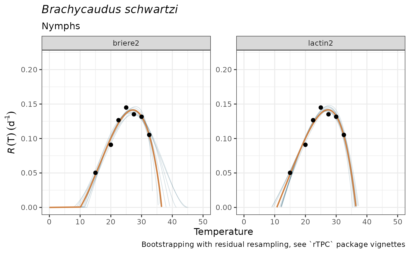

These simulated TPCs may guide ecologically realistic model selection and propagating parameter uncertainty for subsequent analyses. However, as for plot_devmodels(), we discourage selecting among TPC models solely based on statistical information, but rather on informed ecological criteria.

Please, consider carefully whether your data is suitable for these procedures.

References

Padfield, Daniel, Hannah O’Sullivan, and Samraat Pawar. 2021. “rTPC and Nls.multstart: A New Pipeline to Fit Thermal Performance Curves in r.” Methods in Ecology and Evolution 12 (6): 1138–43. https://doi.org/10.1111/2041-210X.13585.

Padfield, Daniel, Hannah O’Sullivan, and Francis Windram. 2025. “rTPC: Fitting and Analysing Thermal Performance Curves.” https://github.com/padpadpadpad/rTPC.

Simmonds, Emily G., Kwaku Peprah Adjei, Christoffer Wold Andersen, Janne Cathrin Hetle Aspheim, Claudia Battistin, Nicola Bulso, Hannah M. Christensen, et al. 2022. “Insights into the Quantification and Reporting of Model-Related Uncertainty Across Different Disciplines.” iScience 25 (12): 105512. https://doi.org/10.1016/j.isci.2022.105512.

Sonderegger, Derek L., and Robert Buscaglia. 2020. “Appendix a : Resampling Linear Models | Introduction to Statistical Methodology, Second Edition.” In. Bookdown. https://bookdown.org/dereksonderegger/570/appendix-a-resampling-linear-models.html.

Woods, H. Arthur, Joel G. Kingsolver, Samuel B. Fey, and David A. Vasseur. 2018. “Uncertainty in Geographical Estimates of Performance and Fitness.” Methods in Ecology and Evolution 9 (9): 1996–2008. https://doi.org/10.1111/2041-210X.13035.

Simulate nn-thermal performance curves using bootstrap with residual resampling

Why propagating uncertainty?

Simulate bootstrapped TPCs with predict_curves()

References

Simulate $n$ -thermal performance curves using bootstrap with residual resampling

Simulate bootstrapped TPCs with `predict_curves()`